
by Olga Klopp
, 06.07.20
With ESSEC Knowledge Editor-in-chief
“Big data”, “high-dimensional statistics”, “predictive analytics” … while we have likely all heard at least one of these terms, their meanings are a little more elusive. How are they applied? How can advances in data analytics impact our daily lives? ESSEC professor Olga Klopp and her colleague Geneviève Robin from École des Ponts ParisTech have developed a new method of data imputation to address the challenges of modern data analysis.
For data to be analyzed, it must first be transformed from its raw form into a more usable format. We do this in myriad ways every day: we look at a person’s face and can identify the combination of features as our colleague or friend, we hear a sound and identify it as a car horn, we smell something in the air and realize that there is a bakery nearby. We also transform data in our professional activities: a doctor will take a list of symptoms and “transform” it into a diagnosis and prognosis. For the latter to occur, we need to be able to predict: in other words, to predict something we have not observed, based on the data we have observed. Think, for example, of a patient who has been in a serious car accident. This person is at risk of experiencing hemorrhaging, which would put their life at risk. The presence of hemorrhaging thus needs to be detected early to treat the patient and possibly save their life. Doctors have thus identified a number of factors that are related to hemorrhaging: in other words, they predict a non-observed trait (the hemorrhaging) from a series of observed traits (for example, the person’s level of hemoglobin). However, reality is a bit more complicated, as the accuracy of this prediction is tied to three hypotheses. Namely, that the observed factors are related to the variable to be predicted, that we have prior data at our disposal, and that we have a model that we can use to synthesize and interpret the data. It is not always possible to verify these hypotheses. Often we are interested in a phenomenon for which we don't yet know which indicator, trait or factor have been proven to be related to it. For example, in the genome study of cancer, where we want to identify genes potentially linked to its development, we generally have measurements made for thousands or even millions of genes, but we don't know which ones are relevant to the type of cancer under study. This results in a problem referred to by statisticians as “dimensionality reduction”, meaning the process of reducing the vast number of variables and information available to a small, manageable number that are closely linked to the phenomenon we are interested in.
For example, say we are interested in three characteristics about a population: height, weight, and a third trait, where we are aiming to predict who has it and who does not. This trait can correspond, for example, to the presence of a disease or a particular symptom. To depict our data, we create a graph, seen in Figure 1, where the horizontal axis represents height, the vertical axis represents weight, and the color of the point represents the presence of the trait. We can see that there is a link between height and weight, where taller individuals are also heavier. We can also see that those with the trait (blue dots) tend to be on the lower end of this and those without the trait (red dots) on the higher end. Because of this observation, we don’t need to know exact height and weight, just where they fall along that line, essentially “summarizing” the information provided by height and weight. This is especially useful because sometimes we may not have all information about an individual at our disposal, so it allows us to “fill in the blanks”, i.e. using data imputation to fill in the missing data. We can then create a third variable that summarizes this information and make the new graph seen in Figure 2: now we have one dimension where before we had two (height and weight). In other words, we have reduced dimensionality.
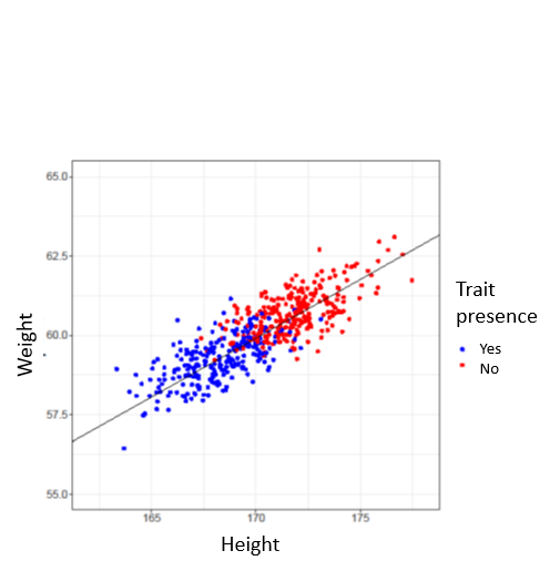
Figure 1. Individuals represented as a function of their height and weight.
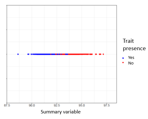
Figure 2. Individuals represented according to their position along the black line in Figure 1.
But what if we need to consider more than two characteristics? Predictive accuracy and value increases with the amount of information included, so data analysts seek to include as much relevant information as possible in their models. Consider the example of a group of people for whom we have seven variables that are related to diabetes, which we want to use to predict if an individual is likely to develop diabetes. Since we have seven variables, plotting these is more complex and harder to visualize than in our previous example. However, by applying the same dimension reduction methods as above, we can create a couple of “summary variables” by looking at the relationships between the seven characteristics and then create graphs with those new summary variables to detect the likelihood of diabetes.
Dimension reduction allows us to take the information at our disposal and synthesize it into a format that can be interpreted more easily. It also allows us, for example, to visualize data, which can be easier to interpret than viewing it in a table. It also increases the accuracy of data imputation methods, which is extremely important in modern data analysis as Big Data is inevitably “dirty” due to missing or inaccurate information. Given the plethora of data at our fingertips, it is also useful for computing, since the summary variables allow for “easier” (less intense and time-consuming) computations. It gives liberty to the analyst, as one is free to choose the number of dimensions (rank) to retain (so long as there are not more dimensions than characteristics). These low rank methods, meaning methods that produce a small number of important new variables from a large number of initial variables are invaluable for modern data analysis.